Gaining an Intuitive Understanding of Bonding Curves
After wading through tons (and tons) of documentation about AMMs and bonding curves I found that some concepts, if I’d understood them at the start, would have made learning so much easier. I’ve collected these observations here, in the hope that it helps others understand how bonding curves work. But before we dive into bonding curves themselves, we need to understand some other terminology and background.
Order Books
When people want to trade something, a common pattern is to maintain an order book. An order book lets buyers record what they want to buy (e.g. Alice wants to buy 100 apples and is prepared to accept 90 pears), and lets sellers record what they want to sell (e.g. Bob wants to sell 90 pears and wants 100 apples). A third party can then use that order book to match buyers with sellers and help perform the asset transfers. This works well so long as you have active lists of buyers and sellers and you can find matches.
Automated Market Makers
An alternative to this order book matching idea has been discussed since the early 2000s. It is the Automated Market Maker or AMM. The idea is that a “pool” is created that contains all the assets that people might want to trade “pre-loaded”. So in our example, we could create an “apples & pears” pool and load it with hundreds of apples and pears. That way, a buyer or seller of either fruit would be able to do their trade directly with this pool, at any time, without having to wait to find a matching order.
The people who fill the pool with the assets are called Liquidity Providers or LPs. They generally deposit lots of both the assets that buyers and sellers want to trade between. LPs can earn a return by taking a percentage of each trade done in the pool. Various pool projects also offer other incentives like bonuses to attract LPs.
Bonding Curves
The idea of AMMs came to the fore again with early blockchain work, Uniswap being one of the early implementations. A thorny question for AMMs was “how can we fairly price the assets in this pool?” and that is answered by using a bonding curve. It is basically a formula, the purpose being to help allow the AMM pool to offer fair prices to buyers and sellers, regardless of their desired trade size and the pool state.
Some Insights
In the below, we’re going to imagine we’re dealing with an AMM pool that can be used to swap back and forth between gold coins and silver coins. These coins of course could represent any on-chain tokens, but for the analogies to work well it’s sometimes helpful to imagine physical coins that we can stack. To make the diagrams easier, we’re going to pretend the silver coins are really high quality and the gold ones are lesser quality, such that initially the coins should trade at 1:1.
1. A Bonding Curve is like a Maze Panel
Imagine you’re in a playground and you see one of those panel things that lets you slide a handle along a curve. The handle is fixed to the rails so can only move where the curve allows it to. It turns out these are called “maze panels” and they can help us form a really useful analogy to a bonding curve.

Imagine the maze panel represents our pool. Wherever the yellow handle is, marks the current state of the pool. The pool state is simply an amount of gold and silver coins. Only the states along the maze panel’s engineered curve are allowed. The pool can’t be in any other state any more than you can move the yellow handle anywhere apart from that pre-defined curve. That maze panel curve is our bonding curve.
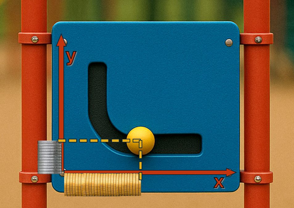
How exactly does the yellow handle represent state? The yellow handle gives us a single (x, y) coordinate, where x represents the amount of gold coins, y the amount of silver coins. We can imagine stacks of coins, representing the tokens in the pool, neatly arranged to run from the edges of the maze panel (the x and y axes) to the yellow handle (the current pool state). We can clearly see how many tokens there are in the pool for its given state:

Or we can draw on some axes and show the same amounts of coins like this:
We can also imagine, if the yellow handle were moved to the left, so that it slid along the curve and upwards, then that new pool state would have fewer gold coins and more silver coins. The bonding curve is never perfectly horizontal or vertical, it’s always got a slight slope. It hard to get that visually accurate in the maze panel photos, but we can imagine.
That leads us to the question, then, how does the pool change state? What can cause the handle to move? The answer to that, lies in how we interact with the pool. We’ve got two main choices:
- When someone trades with the pool (that is, they do a swap) then that yellow handle slides a bit to the left or right, according to which direction the swap was. When someone does a swap, the put in some coins and remove some coins. This causes the heights of the stacks of coins to change and so moves the yellow handle. The size of the trade (the quantities of each coin) affects how far the handle moves. We’re going to look at how trades work in more detail in the next section: ‘You Affect the Price You Get’.
- When someone adds or removes liquidity in the pool, something special happens to the curve shape on our maze panel. We discuss this more in the section ‘The Invariant is Not Invariant’.
2. You Affect the Price You Get
Ok, so now we’re going to look in detail at how a trade (a swap) affects the pool. We know already that trades are going to “move the yellow handle” in our maze panel analogy, but by how far?
Let’s imagine our pool has 100 gold and 100 silver coins so it starts off with an initial pool state of (100, 100). Alice comes along and says “I want to buy some silver, here is 30 gold what will I get back?”. The AMM pool can do a calculation to answer this. The bonding curve is fixed in place, like our maze panel slot, but we can slide along it by +30 coins along the gold (x) axis and see what silver (y) coordinate we will get as a result:
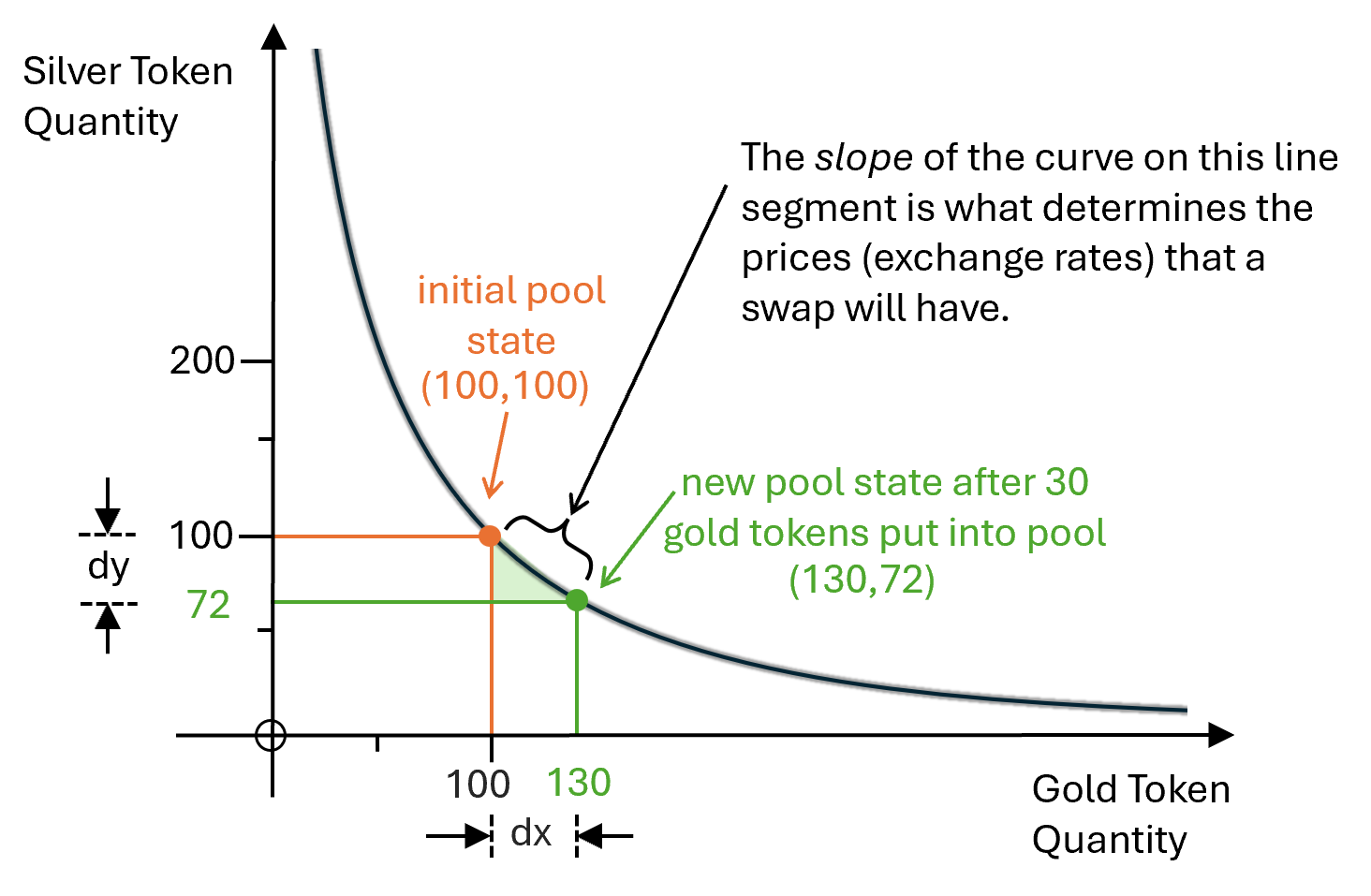
The diagram shows that if we move +30 along the x-axis (dx) we will end up with a y-coordinate movement of 100 - 72 which is -28 (dy). So Alice will get back 28 silver coins.
This is the heart of how AMMs work. Alice, as the trader, can control how big a trade she asks for. If she were to say she wants to spend 300 gold coins, we’d end up sliding along the x-axis for a long way, but we’d only move a relatively short distance on the y-axis. So Alice would get a really bad deal on a gigantic trade that adds lots of gold.
Alice’s better strategy would be to do multiple small trades, and hope other traders take the opposite swap direction in between. The closer the yellow handle is to the centre of the chart, the better the price is for everyone.
If Alice did decide to spend 300 gold on some silver, regardless of the fact she’d get a bad deal, then what would happen? The yellow handle would move way to the right of the curve, and then other traders are incentivised to move it back to the centre again, to go the opposite way, because the pool would be offering an awesome deal on purchases of gold. Alice would have made the pool “gold heavy” and that means using a small amount of silver to buy gold would get us a great deal. Our pool’s customers are incentivised to bring the pool back to balance again.
3. The Invariant is Not Invariant
As already mentioned, Liquidity Providers (LPs) pour in pairs of tokens to AMM pools. In our sample pool of gold and silver coins, we expect it to start off balanced and to trade at around 1:1 when the pool starts up.
What is interesting, though, is what happens to our maze panel curve when an LP adds pairs of tokens to an AMM pool after that initial deployment. As mentioned, a bonding curve is just a formula. For example, Uniswap use the famous constant product formula x.y = k which says that the quantity of gold coins times the quantity of silver coins must always equal the constant k. This value k is often called “the invariant” and the formula itself is called “the invariant formula”.
But here’s the insight, the invariant k is not invariant when an LP adds or removes liquidity. When an LP adds more liquidity the value k increases, because we have more gold coins and silver coins to go around. If an LP removes liquidity we have less to go around, and k has to decrease. The invariant k is only really invariant during swaps. Note however, that the bonding curve formula remains the same (x.y = k in this example), it’s just that one of the parameters is changing.
Here’s a diagram of how the curve (aka our maze panel slot) changes as more liquidity is added:
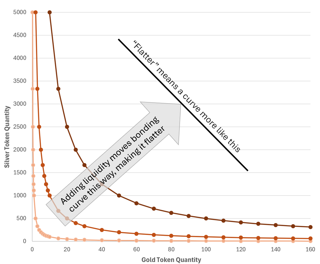
We can see the curve “flattens” as more liquidity is added. Crucially, a flatter curve means a better price for both buyers and sellers, so a pool with a lot of liquidity is a good thing. The more coins LPs put in, the better it is for everyone trading. Remember that during a trade, it doesn’t matter where in the xy plane we are, what matters is the slope of the curve because it is the slope of the curve that determines the prices.
4. AMM Projects Determine Bonding Curve Shape
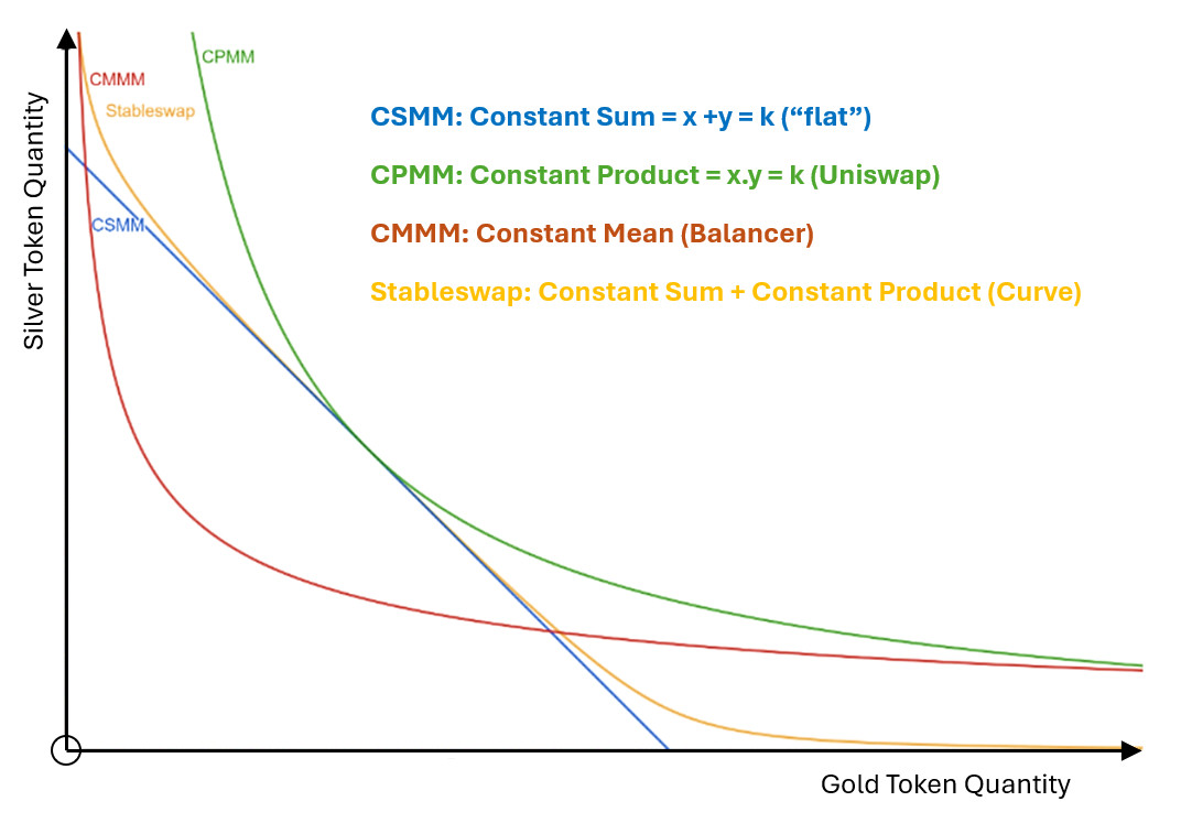
The bonding curve shape, aka the maze panel cutout shape, also varies by AMM project. Different projects offer different curve formulas and different parameters you can tweak to alter the shape to suit your use case.
For example, tokens that we know should trade at very close to 1:1 always, like pairs of USD stablecoins, benefit from having a “flatter” bonding curve in the middle. This is shown in the diagram below by the yellow line, from the Curve project’s Stableswap bonding curve.
5. Curve StableswapNG Parameters
Different AMM projects allow you to tweak their curve in different ways. For example, Curve’s StableswapNG pool offers several parameters to tweak their curve to suit your preferences. The parameters are shown below, along with samples of what some existing large pools use there:
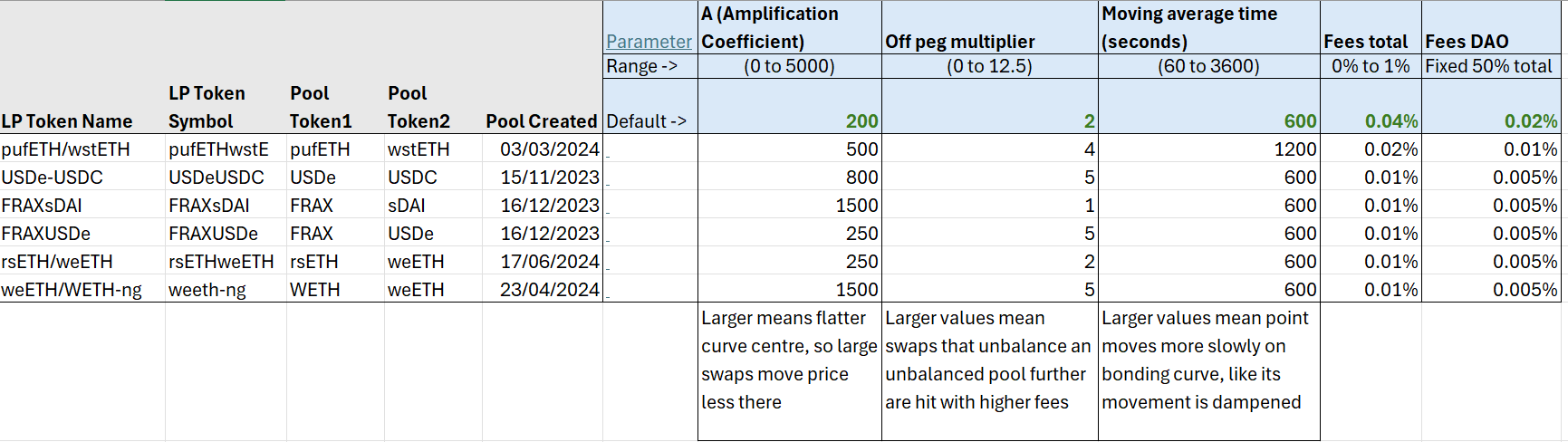
- A = Amplification Coefficient. Range 0 to 5000. Larger values mean flatter curve centre, so large swaps move price less there.
- Off peg multiplier. Range 0 to 12.5. Larger values mean swaps that unbalance an unbalanced pool further are hit with higher fees.
- Moving average time. Range 60 to 3600 seconds. Larger values mean point moves more slowly along the bonding curve, like its movement is “dampened” across time.
That’s it for now! I’ve collected material for a “bonding curves part 2”, where we can extend our understanding to concentrated liquidity, oracle integration and tri-pools but that’s for another day.